The “September Case”: Myth or Reality?
September has always been one of the most feared months by investors.
You may have heard of it—a negative trend that seems to hit the stock markets right around this time every year. But how true is it? And more importantly, how can we protect ourselves?
In this video, we’re going straight to the point. We’ll dive into historical data to find out whether this “September effect” is just a myth or if it’s actually backed by numbers. And if it is, we’ll explore a simple strategy to face the month with more awareness and less risk. In other words, a kind of hedging strategy.
So let’s skip the small talk and, as quantitative traders, get straight into the numbers.
Analyzing 25 Years of Data with Bias Finder
Alright, let’s start right here with this screen. What you see is the Bias Finder—one of the proprietary software tools developed by Unger Academy. What does this tool do? It helps us analyze various biases—those recurring trends we see in historical price data.
Specifically, we’ve got intraday bias, weekly bias, and monthly bias. But for today’s video, we’re interested in the annual bias—more commonly known as seasonality.
In this case, I’m going to load S&P 500 data—the S&P 500 futures—from the year 2000 up to the present day. And I’ll calculate the bias as a percentage.
Another thing we can do is break this time period into smaller segments. In this example, I’ll split it into two parts: from 2000 to 2010—what we might call the “dark decade” marked by two recessions—and from 2011 to 2025. So, let’s go ahead and calculate the seasonality.
Alright, here it is. The blue line you see represents the average total return of the S&P 500 from 2000 to today across the calendar year. The yellow line shows the average return from 2011 to today, while the red line reflects the average from 2000 to 2010.
The Market’s Weak Spot? From Mid-September Onward
One thing that immediately stands out is that, as you can see, the red line generally shows lower returns compared to the yellow one. That lines up with what I mentioned earlier—2000 to 2010 was a tough period, shaped by two recessions.
Alright, now that we’ve set the stage and understood how everything works and what we’re looking at, let’s dive a bit deeper. Specifically, let’s focus on this time window—from September through October.
One interesting thing that jumps out right away is that September really does come across as a negative month. You can see it clearly in the blue line, and it’s also confirmed by both the yellow and red lines. In fact, whether we’re looking at the more “positive” period, so to speak, or the one marked by the two recessions, September still shows up as generally negative.
So, it looks like this negative trend that tends to worry investors is actually confirmed by the data, just like we’re seeing here.
However, what I’d like to do now is zoom in on this window even further. I mean, yes, the whole month of September is roughly negative—but is there a specific day where it makes more sense to go short? Just by eyeballing the chart, you might notice it starts around mid-September.
Putting the Pattern to the Test
At this point, let’s switch over to MultiCharts and take a closer look at this part.
Here we are in MultiCharts. I’ve loaded the S&P 500 futures using daily data going back to around 1990 or 2000—basically, the full dataset we have available. Since we’re working with seasonality, the sample size is unfortunately a bit limited. That’s why we try to include as much data as possible.
In this case, I built a very simple strategy, and I’ll walk you through how it works. First, I set up an input called “start window,” which I initially assigned a value of minus one. We’ll see why in just a second.
Then we have two conditions. Condition one is that the month must equal nine—which, in plain English, just means we’re in the month of September.
Condition two says that the calendar day must be greater than or equal to our input. In other words, we need to be within the window we’ve defined for taking short positions.
As just mentioned, this strategy is designed to go short—so if both condition one and condition two are met, we’ll open a short position on the next bar in the market.
As for exits, to keep things simple and just get a feel for how this strategy performs—or whether it has any potential at all—I used a basic “set exit on close.” That means all positions will be closed at the end of the session.
Alright, let’s go back to the chart now and take a look at this strategy, which I’ve already added. As you can see, it just takes a quick check of the box here, and we can see how it works.
Okay, so here we’ve got a whole series of trades. When are these trades triggered? From the beginning of September to the end of September. Why? Because in this case, the input is still set to minus one.
So if you remember how we coded it, the time window condition is: greater than or equal to minus one. Basically, every calendar day in September is greater than or equal to minus one, which means we’re trading throughout the entire month of September.
Now, some of you might be wondering why I chose to use “set exit on close”—in other words, why open and close a position every bar, instead of, say, opening a trade at the start of the window and holding it until the end?
That’s a valid question. The reason I did it this way is because I want to go in later and analyze whether there are more efficient entry and exit points.
So what I’m aiming for here isn’t really a kind of position trading strategy where I hold a position through the full seasonal window. Instead, I’m thinking of more of a trading system where I can make multiple entries during that window—possibly using different criteria for entry and exit. We’ll dig deeper into that in just a moment.
Let’s start by looking at the performance with a single contract. As you can see from the equity line, we’re already off to a pretty solid start. It’s clear that, on average, September has been a negative month—which aligns nicely with what we saw earlier in the Bias Finder.
Looking at the total trade analysis—specifically the number of trades and the average trade—we can see that there are 582 trades, and the average trade is around $75. For this instrument, considering we’re trading short and doing intraday trades, that’s a very good starting point.
Optimizing the Trading Window
Now let’s try to understand in more detail how we can get the most out of this seasonal window. And what I want to do now is run an optimization.
Specifically, an optimization of the start of the time window. So instead of beginning on the very first day of September, maybe it’s more effective to start trading on the 10th, or the 15th, and so on.
Unfortunately, I don’t know the answer just yet—or rather, I can at least try to get an idea of what the best result might be by going back to the analysis we did using the Bias Finder.
If you remember, in the Bias Finder we saw that there was a clear drop starting around mid-September. So I expect that, even in this case, if we run an optimization, the best results will probably start showing up around the 14th or 15th of the month. Let’s find out. We’ll run the optimization from -1 to around 30, which covers all 30 calendar days.
Alright, here we have the results—this is the table view. But we can also visualize it with a chart, which might be easier to interpret. And what jumps out right away is that if we start trading right at the beginning of September, we get a higher net profit. But that doesn’t necessarily mean it gives us the best average trade. We’ll see that more clearly in a moment.
Then, as we narrow the time window, we notice that the net profit drops—until, just as I mentioned earlier, starting from mid-September, there seems to be a stronger edge in shorting the market.
Just to tie this back to what I was saying earlier—why would I choose a value from this range here, rather than something like 0, 1, or even -1? Well, we can see that clearly in this tab.
If we take -1 as a reference point—the same value we were using before—it gives us a net profit of $43,000.
Pretty close to, say, a value of 16, which gives us about $41,000. So, not a big difference in net profit. But what is interesting is the average trade.
Because while the -1 setting results in a higher net profit, the average trade is only $75. In contrast, if we choose 16, the average trade is almost double what we get with -1.
And that’s exactly why I’d go for one of the values in this range here—most likely 16, which seems to give us the best average trade among the nearby values. So let’s go ahead and select 16.
Okay, and as you saw, it immediately kicks in here. Basically, instead of starting to trade on the first day of September, we now begin around mid-September and trade through the end of the month. So yes, we’ll be placing fewer trades, but as we saw earlier, the net profit stays roughly the same—and the average trade increases.
Let’s take a look at the performance now. As you can see, the equity line looks really good—very smooth, steady, and quite similar to the one we saw earlier. If anything, maybe a little “cleaner” in the middle section—but overall, we’re in the same ballpark.
What I especially like about using this new input—this reduced time window—is that we end up with a significantly better average trade.
So again, we’re looking at a strategy that gives us some very promising results. It’s not quite ready to go live yet, though, because we’re not managing risk properly. What I mean is, for example, there’s no stop loss in place. And I’m pretty sure we could get even better performance by improving either the entry or the exit.
Improving the Exit: Dynamic Take Profit
Let me show you an example. Here, back in the code, we’ll leave everything as it is but try changing the exit condition. So instead of using just the set_exit_on_close, let’s try exiting based on a kind of take-profit rule—something tied to the low of the previous session.
So, by writing this simple line of code, what I’m basically doing is closing the short position as soon as the previous session’s low is broken. Let’s compile and see how that changes the trades.
At first glance, it might not look like much has changed—but if we zoom in a bit, like on this bar here, you’ll see that we enter the short position at the open, and then we close it once the previous session’s low is broken.
So, just to recap, we’re not exactly setting a take profit, but in a way, we are locking in some gains. Let’s take a look at how the strategy changes.
And right away, you can see that this small change really cleaned things up. The equity line now looks much smoother and more consistent. We can also see that net profit has improved—from about $45,000 before to $46,000 now. And when we check the average trade, that’s also gone up—from around $138 per contract to roughly $155.
Does It Work on the Nasdaq Too?
But I decided to take it one step further. It’s true that this strategy works really well on a future like the mini S&P 500—but now I’m wondering: how does this exact same strategy perform, using the same input—specifically the 16th day for the start of the time window—and the same exit logic, on a correlated future like the Nasdaq?
In this case too, I expect the results to be more or less the same. Why? Because these are two instruments that move very similarly—they’re both stock index futures. And if the results on the Nasdaq didn’t align with what we saw on the S&P 500, then yeah, I’d start to question things.
So, as you can see, I’ve already applied the strategy to the Nasdaq future. Let’s change the input value to 16 and see how it performs.
Looking at the equity line, the overall behavior is pretty much identical. The net profit is actually slightly higher—looks like about $2,000 more—and the average trade is around $176. That’s partly because the Nasdaq tends to be more explosive compared to the mini S&P 500.
But the important takeaway here is that the performance confirms the edge we found for the month of September. It’s not just something that randomly worked on the S&P—it holds true for the Nasdaq as well.
Next Steps and Potential Improvements
So, where could we go from here? Like I mentioned earlier, the next logical step would be to add a stop loss—try optimizing it and figure out what the best value might be. Or we could work on the entry conditions.
Right now, as you’ve seen, we’re using a daily time frame and we enter a trade simply because we’re within the defined time window.
But what we could do is use a lower time frame, and instead of entering right away, wait for a specific level to break—either in a mean-reverting or trend-following fashion. Or maybe we add some filters—volatility filters, price patterns, or whatever else you believe is appropriate.
Final Thoughts
Alright, so in this video we’ve shown, with data, that September really is a month marked by a negative window. But not only that—we’ve pinpointed exactly when it tends to start, around the 16th day of the month, and we’ve looked at how to profit from it—or at least build a solid hedging strategy to operate during that time.
That’s it for today.
As always, if you’re interested in this kind of content, you’ll find more useful info by clicking the first link in the description. And I’ll see you in the next video.