Different Ways to Use Moving Averages
I’m pretty sure that if I asked you to name some indicators used in trading, one of the first that would come to mind is the moving average. We’re talking about one of the most well-known tools in technical analysis, appreciated specifically for its simplicity.
In fact, it’s just an arithmetic average calculated over a given number of periods, a very simple mechanism, yet one that can have some very interesting applications.
As often happens in these cases, over time various versions have been developed, from exponential to weighted moving averages, and so on. But in this video, we’ll be focusing on the simplest of them all: the simple moving average.
We won’t just look at how it appears on the chart. We’ll also explore how to use it as an operational filter and to determine what kind of market regime we’re in.
And this brings us to an important side note: what do we mean by “market regime”? Quite simply, it’s the current phase a market is in at a given moment.
It can be an upward regime if prices are rising, a downward regime if prices are falling, and so on. So, at this point, I’d say let’s switch to the chart and move forward with our analysis.
Approach 1: 200-Period Simple Moving Average
Here we are. In this workspace, I’ve placed three charts where moving averages are used in three different ways to understand which market regime we’re currently in.
The first point I want to focus on is how I chose the calculation period for the moving average. Honestly, nothing too complicated. I just went with the most commonly used values—basically, the default settings you typically find on most trading platforms.
In fact, typically when trying to understand what kind of market regime we’re in, the most widely used moving average is the 200-period moving average. Next, the 50-period moving average is commonly used.
So now that we’ve cleared that up, let’s dive into the first chart. Here you can see a 200-period moving average, which is the red line.
The interpretation here is pretty straightforward: if the price is above it, we’re in a bullish market regime. On the other hand, if the price is below it, we’re in a bearish regime.
In this specific example, I’ve used SPY, the ETF that tracks the S&P 500. And you can clearly see that during the 2008 crisis and recession, the 200-period moving average acted as a great filter to show we were in a bearish regime.
So, what can we say about this approach before we move forward with the analysis? It’s certainly a very simple one (we’re only using one indicator), and it lets us understand relatively quickly whether the market regime has changed.
Approach 2: Crossover Between the 200 and 50-Period Moving Averages
Of course, this is in comparison with the next two methods, the other two approaches that we’re about to look at. In fact, in the second approach, which you can see here, we’re now using two moving averages. This time, it’s all about the crossover between these two moving averages: the 200-period moving average, which is the blue line, and the 50-period moving average, shown in pink.
In trading literature, or more commonly in trading lingo, this setup gives us what’s known as the “Dead Cross” or “Golden Cross.”
Dead Cross and Golden Cross
What are the Dead Cross and the Golden Cross? The Dead Cross occurs when the 50-period moving average crosses below the 200-period moving average, and the Golden Cross is the opposite—when the 50-period moving average crosses above the 200-period moving average.
Naturally, the names given to these two crossovers help us understand what the market is expected to do after such a crossover occurs.
That is, when we see a bullish crossover, we’re likely entering a bullish market regime. Conversely, when we see a bearish crossover, like the one shown here during 2022, we’re likely in a bearish market regime.
So, once again, analyzing this with a bit of objectivity, what can we say about this approach? It’s definitely a bit more complex than the one we looked at earlier, because in this case, we’re waiting for a crossover between two moving averages.
So by definition, since a moving average is already a lagging indicator, meaning it gives us a delayed signal, this setup gives us an even more delayed signal, because instead of just waiting for the price to cross the moving average, we’re waiting for two moving averages to cross each other.
That said, what’s immediately noticeable is that this signal is still very clean and clear to interpret. So this approach, too, can be very useful when identifying the market regime.
Approach 3: Slope of the Moving Average
Alright, let’s now move on to the final approach, probably the least well-known and least discussed one, but I still wanted to show it to you because I think it’s a very interesting method.
In this case, I’ve once again used a 200-period moving average,
but you’ll notice that its color changes. The signal, in this case, doesn’t come from the price position relative to the moving average,
nor from a crossover with another moving average, but instead from whether the color is green or red.
Naturally, green indicates a bullish market regime, while red indicates a bearish market regime.
So, how did I determine the color, or in other words, the market regime we’re in?
I calculated the slope of this moving average over another reference period, in this case, 50, referring back to the widely-used 50-period moving average.
Let me explain a bit better. What do I mean by “slope”? Let’s try to understand this by looking at the moment when the moving average changes from green to red.
Very simply, imagine drawing a line connecting the current value of the moving average to the value it had 50 periods ago. If this line has a negative slope, then from that point onward, we’re in a bearish regime.
On the other hand, let’s say I randomly pick a point over here, and I draw a line connecting it to the value observed 50 periods earlier, if that slope is positive, then in that case we’re in a bullish regime.
So, what can we say in this case as well? That it’s a slightly slower signal compared to the first method we saw, the one where we simply check where the price is in relation to the moving average.
And in fact, we can clearly see it right here. Here we have the crossover of the moving average. However, the market only enters a bearish regime from this point onward, when the line turns red.
On the flip side though, just like in the second example we saw,
with the crossover between two moving averages, even here, the signals appear quite clean and easy to interpret, which means they could be used as an operational filter.
Effectiveness Testing on a Portfolio of Instruments
Great, now that we’ve covered this little bit of theory, let’s—as always try to figure out quantitatively which of these three methods might be the best for determining what market regime we’re currently in.
To do that, we’re going to use the Portfolio Trader. And what does the Portfolio Trader do? Well, just like the name suggests, it applies a strategy to a portfolio of instruments.
In this case, I created a fairly diversified portfolio that includes a number of different ETFs, like the S&P 500, the Nasdaq, and many others, such as Growth stocks, emerging markets, Gold ETFs,
Bond ETFs, Silver ETFs, and so on. So, as I mentioned earlier, the goal was to create a well-diversified portfolio.
The Trading System Used for the Test
Let’s now take a look at the script we’ll be using, so we can better understand how it works. First of all, you’ll see an input field, which is labeled “type”.
If the type is set to 1, we’ll be using the first approach we looked at, the one that checks the closing price in relation to a 200-period moving average. So just to be clear: this is the one where we observe the price relative to that red 200-period moving average.
If the type is set to 2, we’re using the second approach, that is, the crossover of a 50-period moving average with a 200-period moving average.
Finally, as you can imagine, type 3 corresponds to the method
where we analyze the slope of the 200-period moving average.
Let’s go back now to the Portfolio Trader. Great, let’s launch an optimization focusing on just one input: the type.
By setting it to vary from 1 to 3, we’re basically simulating
the three different approaches we’ve analyzed so far. And this allows us to evaluate their results when applied to our portfolio.
At this point, I’d say let’s go ahead and launch the optimization.
And here is the report that’s been generated. Just to clarify once again: Type 1 is the approach where we take the 200-period moving average and compare it to the closing price.
Type 2 is the crossover of the two moving averages. And finally, Type 3 is the one where we analyze the slope of the 200-period moving average.
Comparison of the Results from the Three Approaches
So, what can we say about this report? Well, if we were to look only at net profit, we can see that the approach using the crossover of the two moving averages is the one that delivers the highest return.
But let’s not limit ourselves to just the net profit, let’s also take a look at the other metrics provided in the report. First, let’s examine what happens with the Max Intraday Drawdown, so the drawdown that occurs when we simulate these three approaches on our portfolio.
We can see that with the crossover of the two moving averages and with the slope of the moving average, the drawdown is around $27,000 and $28,000. Given the simulated capital for this portfolio is $100,000, that equals roughly a 27–28% drawdown.
On the other hand, if we look at the simplest approach, the one where we use just a single moving average and analyze where the close is in relation to that moving average, we see that the drawdown in this case is significantly lower, sitting at around 18.6%.
Okay, let’s move forward with the analysis because there’s something else interesting when we look at these two columns: Total Trades and Percent Profitable.
So, what does Total Trades represent? It’s the number of trades that are executed with that specific approach. And Percent Profitable is simply the win rate: how often a trade ends in profit compared to how often it ends in loss.
And here we can clearly see that with the first approach, the one with the close in relation to the moving average, a much higher number of trades is executed compared to the other two methods.
We’re looking at around 1,000 trades versus 150 and around 100.
Now, analyzing the Percent Profitable, we can see that the win rate is about 27%, which is quite low. Just imagine: out of 10 trades, only 2.7 are closed in profit. With the other two approaches, though, we’re roughly around a 50/50 win-loss ratio.
Alright, so let’s try to put these results into context and understand what’s going on. Why does the first approach generate so many trades, while the other two produce so few?
Well, it’s because, just as we’ve seen in the earlier examples, the method that uses the moving average crossover as a reference
gives us a very clear and, let’s say, “clean” signal. As you can see here, once the crossover happens, we don’t get another one for several months.
On the other hand, if we look at the first method, where the price is crossing above and below the moving average, you can clearly see that there are multiple cases where the price is above one day, below the next, then back above, and so on.
Just to visualize it better, let’s apply the strategy with the type set to 1, meaning we’re using the close relative to the moving average. And here, you can see how many entries are generated in this scenario.
Now, imagine a case where the signal only triggers when one moving average crosses another. Clearly, the number of entries would be much lower, and that’s exactly what we’re seeing in this report: 1,000 trades versus just 150 and 100.
However, as you can see when analyzing the drawdown, it’s much lower with the first approach than with the other two. Why is that? Because the signal simply arrives sooner.
We already looked at this earlier, for example, in this specific case. Here, to determine that we’re in a bearish market regime, we didn’t base it on the crossover with the close, but we had to wait for the moving average to cross below the 200-period moving average. And clearly, a lot can happen during that time.
Now imagine there’s a sudden, violent crash. In our backtest, that would translate into a larger drawdown when using that type of approach.
What’s the Best Way to Use Moving Averages?
So, to give a sort of final answer about which of these three approaches is the best, I believe we first need to consider how we plan to use them.
Let me explain. If I were to use these three approaches solely and exclusively as a trigger, meaning I build a trading system that simply takes the moving average crossover as the entry point, then I would also need to analyze the average return per trade, for each of these three approaches.
Because the first approach will definitely have a much lower average trade compared to the other two. As you can see, we’re looking at a similar net profit, but with ten times more trades. So it’s safe to expect that the average trade is also about one-tenth of the other two approaches.
Now, if I had another strategy, one that, for example, goes long or short based on other rules, and I were just using the moving average as a filter to understand what market regime I’m in, which of these approaches would I use? I would definitely choose the first one, because it allows me to operate with lower drawdown.
So basically, I’m able to realize more quickly that the market regime has changed. Now it’s true that the number of trades is much higher,
and as a result, the average trade is lower, but that’s not what matters in this case, because, as I mentioned, I already have another strategy that handles the actual trading in different market regimes.
I understand this is a fairly broad topic, and of course, it also comes down to personal preference, but I’ve brought you an example here just to illustrate what I mean.
Testing on SPY and TLT ETFs with Larry Connors’ Strategy
So here I’ve used two of the ETFs we looked at earlier, SPY and TLT, to include both a stock ETF like the S&P 500 and a U.S. bond ETF.
To these two ETFs, I applied a well-known strategy that’s been out of sample for around fifteen years now.
It’s a strategy developed by Larry Connors, a well-known author and systematic trader, that uses the RSI indicator, the classic oscillator we often refer to, set with a 2-period calculation.
Let’s now break down the code for this strategy so we can see exactly what it does. First of all, I’ve also used an input in this case.
And what does this input do? If it’s set to 0, we won’t apply the moving average filter to determine what market regime we’re in. But if the input is set to 1, as you can see, we’ll use the moving average to filter the trades accordingly.
So, the base strategy, as you can see, is very simple. We have the RSI again with a 2-period setting. If it crosses below level 5, we buy. If it crosses above level 95, we open a short position.
And when are these positions closed? When the price crosses a 5-period moving average, which is a very fast moving average.
Now let’s understand what happens when we vary the input from 0 to 1, and how that changes the behavior of the strategy by allowing it to trade only under certain market conditions.
As you can see, if I set the input to 1, then I’ll only take long trades when the close is above the 200-period moving average, and I’ll only enter short trades when the close is below the 200-period moving average.
Alright, let’s go ahead and analyze the reports. Here you can already see that I’ve set the input to 0, so the moving average filter is not applied.
In fact, you can see that here we are roughly at the market highs, yet short entries are still being made.
Now let’s analyze the performance. Here we see an equity line that is overall quite positive, with a fairly steady upward trend. Sure, there are some drawdowns, but all in all, it’s a good starting result.
Looking at the long side, it obviously performs much better, especially considering the underlying trend of this instrument, which in this case is the S&P 500. When we look at the short side, it struggles a bit more, but overall, as you can see, we still get positive returns.
Okay, now let’s analyze the same system on TLT. Here again, you can see that even though we’re at a much lower level, long entries are still being made, because we’re not applying the moving average filter.
Analyzing performance here as well, we see an equity line that’s less consistent compared to the one we saw earlier. On the long side, we see a fairly deep drawdown, but over the years, the overall performance has been relatively steady.
It’s a bit of a different story on the short side, where we see an even deeper drawdown, specifically around the 2019–2020 period.
Using Moving Averages as a Filter Within a Strategy
Alright, now let’s go ahead and apply the filter to both strategies. So, I just need to set this input to 1.
And here it is. As you can see, for example, we’re no longer entering short trades right near the market highs. But if we zoom in for a second, we see that short trades are only executed here in this phase in 2022, when the price was below the 200-period moving average.
Great, let’s analyze performance here as well, and now we can see that the equity line is much more consistent. As for the long side, the trend remains positive, partly because, as mentioned earlier, that’s the underlying trend of this asset.
On the short side, if you remember, even though it was struggling earlier, now you can see that while not many trades are executed—
because it’s rare for the market to be in a bearish regime compared to its long-term trend—even here, the performance is smoother.
Now let’s analyze the same strategy with the filter applied to TLT. So once again, I’ll set the input to 1. And of course, here too, we only get short entries in this phase, because the price is below the moving average, and long entries only here, because the price is above the moving average.
Now, looking at the total equity line, you’ll see the situation changes completely. Now the equity curve is much more stable both for the long side—remember, there was a significant drawdown here,
which no longer happens—and also for the short side.
And so, in cases like these, a 200-period moving average,
even though it generates more signals than the other two approaches—the crossover of two moving averages or analyzing the slope—if used as a filter in a trading system, can really deliver great results.
Final Thoughts
In this video, we looked at how to use moving averages starting from their simplest form, and exploring how they can be applied to identify the current market regime.
As mentioned earlier, there are many other types of moving averages
that can be calculated not only on closing prices, but also on values like open, high, or low. And of course, that’s not all.
We can also apply them to variables that have nothing to do with price, like volume, macroeconomic indicators, or other market data.
There are truly so many possibilities, and if you’d like to dive deeper into any of these topics, let me know in the comments.
But for today, that’s all. See you in the next video.