Hey everyone, I am one of the coaches of Unger Academy and I’d like to welcome you to this brand new video.
Today we are going to continue talking about spread trading.
In the first video – here on top you can find the link to watch it – we talked about the spread between two futures, the US and the TY, that is, the thirty-year and the ten-year US bonds.
But before we go any further, if you haven’t had a chance to take watch it yet, I invite you to go and check it out. You might find some interesting ideas in it. Plus, it’s very important because, otherwise, you wouldn’t understand what comes next in this video. So the link is here on the top.
Today we’re going to be figuring out on which other futures pairs it would be possible to use this kind of strategy.
Futures spread portfolio
Okay, as you can see here, I added several strategies to the initial portfolio, in addition to those on the two bond futures. In particular, I have applied the ‘steepening‘ and ’flattening’ approach to the other futures pairs. The code used for these strategies is the same that I’ve shown you in the first video about spread trading, but now it’s obviously applied to different markets. If you want to see how the code is written, I recommend watching the first part of the video.
Here we see Mini S&P 500 and Nasdaq, which are two correlated markets. Then we have Crude Oil and Heating Oil, so two energy futures, and finally, Silver and Gold, two metals futures.
Now these markets are characterized by a high degree of correlation, in a purely statistical sense, and a fairly similar notional value (that’s the countervalue). Now, I hope the spread trading purists will forgive me, I mean, they’ll probably say that this is not enough and that we should do further tests to identify the actual degree of correlation and integration between these markets. However, my purpose is just to build some very simple trading systems that retail traders can easily use.
By making simple multiplications, we can see that the value of these pairs is quite similar. Take the S&P and the Nasdaq, for example, which you can see here on the top left. The value of S&P is about $220,000, that is, $50 (the value of one point) multiplied by the last close (about $4,400). And the notional value of Nasdaq is about $298,000, that is, $20 (the value of one point) multiplied by the close, which is $14,700.
The US and the TY also have similar notional values. In fact, both markets have a Big Point Value – which is the value of one point – of $1,000.
So, the value of one contract of the TY is $131,000, and the value of one contract of the US is $157,000.
Gold and Silver also have similar notional values (although their volatility levels are different), and the same thing applies to Crude Oil and Heating Oil. Their notional values correspond to $80,000 and $105,000, respectively.
In short, the notional values of the various contracts are similar, and this is something we can exploit without going into particular details.
I added all the pairs we’re going to work with to this workspace. So we have ES-NQ, US-TY, GC-SI, and CL-HO. As you can see, all the strategies make opposite trades. For example, when there’s a long position open on Mini S&P500, there will be a short position on the Nasdaq, and the same goes for all the other pairs.
Portfolio test
At this point, we can go back to MultiCharts Portfolio Trader and test these pairs to see what effects we get.
When we run the test on our portfolio, we immediately see that the average trade is lower than the one we got when we tested the strategy only on the US-TY pair. Keep in mind that the average trade is essential in this test since by opening two positions at a time, slippage and commission costs have a greater impact on the portfolio.
So now the average trade went from about $130 to about $50. Perhaps, this dramatic decrease means that not all the pairs in the portfolio are suitable for spread trading or, at least, for this spread strategy, which uses a moving average calculated on the spread itself as a filter.
If you have any ideas to filter this strategy in any other way, please just let us know in the comments. It’s greatly appreciated.
Going back to our backtest, we can see that there are losing pairs and pairs that perform pretty well. As we already know from the first part of this video, the US and the TY do perform well. The ES-NQ pair also produces good results, with a total profit of about $45,000.
The other pairs, however, either lose money or make irrelevant profits. Take a look at Crude Oil and Heating Oil. Quoting Shakespeare, there’s “much ado about nothing” here. I mean, there’s a huge amount of trades that generated huge profits and losses, but in the end, they didn’t bring any real benefit to the portfolio.
And as for Gold and Silver, they even produce negative results.
So, is it possible that our spread trading strategy can only be used on a few financial instruments? Such as stock indexes and bonds? The results we obtained in our test suggest that it is possible.
Let’s take a look at the overall equity line. It is still positive, but not without some very significant shocks. As you can see, it would be very difficult to go live with this portfolio. Nevertheless, it is possible to play with the filters or optimize the existing ones, that is, those using the moving average period to separate steepening and flattening moments.
Conclusions
Also in this case, there are several possibilities for further development. And you know, the purpose of this series of videos is precisely to arouse your curiosity about the creation of new automated strategies.
And this is what we teach at Unger Academy – a method to become fully autonomous in building your own trading systems.
In this regard, in the description of this video, you can find a link to a webinar. If you have already watched it, go ahead. If you haven’t, please go and check it out. It’s free and provides a clearer picture of how to become an autonomous trader.
And that’s it for this video.
Thank you so much for watching! Will see you soon! Bye-bye!